优化 - 数据预处理
优化训练模式,并且处理非数字数据
Optimization
微调管道内部,超参数优化
Hyper-parameters optimization
构建管道和准备数据
构建管道
from sklearn.pipeline import make_pipeline
from sklearn.linear_model import SGDClassifier
from sklearn.preprocessing import MinMaxScaler

pipe = make_pipeline(MinMaxScaler(), SGDClassifier(max_iter=1000))
2
3
4
5
查看管道参数
print(pipe.get_params())
准备数据
from sklearn.datasets import load_digits
from sklearn.model_selection import train_test_split

X, y = load_digits(return_X_y=True)
X_train, X_test, y_train, y_test = train_test_split(X, y, stratify=y, random_state=12)
2
3
4
5
GridSearchCV 调优
使用GridSearchCV搜索当前训练集下的最优参数
# 使用网格搜索找到当前训练集下最优参数
from sklearn.model_selection import GridSearchCV
import pandas as pd

param = {'logisticregression__C': [0.1, 1.0, 10],
         'logisticregression__penalty': ['l2', 'l1']}
grid = GridSearchCV(pipe, param_grid=param, cv=3, n_jobs=1, return_train_score=True)
grid.fit(X_train, y_train)
print(grid.get_params())
2
3
4
5
6
7
8
9
- 这里要调优的参数为
C和penalty,需要在param手动中写明 - 注意这里的
grid就是一个机器学习模型,和管道pipe,分类器clf相同 - 只有当
grid已经经过训练,并且调用了score函数后,其最优函数才会确定下来,否则不认为当前训练集已经结束
查看各参数对训练的影响以及结果
df_grid = pd.DataFrame(grid.cv_results_)
print(df_grid)
2
   mean_fit_time  std_fit_time  mean_score_time  std_score_time param_logisticregression__C  ... split0_train_score split1_train_score  split2_train_score  mean_train_score  std_train_score
0       0.126961      0.001999         0.006072        0.007825                         0.1  ...           0.949889           0.953229            0.949889          0.951002         0.001575
1       0.247481      0.017783         0.000620        0.000040                         0.1  ...           0.891982           0.909800            0.904232          0.902004         0.007442
2       0.425019      0.011945         0.000617        0.000032                         1.0  ...           0.989978           0.988864            0.984410          0.987751         0.002406
3       1.135990      0.046367         0.000678        0.000057                         1.0  ...           0.982183           0.982183            0.979955          0.981440         0.001050
4       1.080702      0.094789         0.000640        0.000035                          10  ...           0.998886           0.998886            0.998886          0.998886         0.000000
5       5.193207      0.190867         0.000609        0.000019                          10  ...           1.000000           1.000000            1.000000          1.000000         0.000000

[6 rows x 18 columns]
2
3
4
5
6
7
8
9
查看当前训练集下最优的C/penalty
print(grid.best_params_)
{'logisticregression__C': 1.0, 'logisticregression__penalty': 'l2'}
对模型grid进行精准度测试
accuracy = grid.score(X_test, y_test)
print('Accuracy score of the {} is {:.2f}'.format(grid.__class__.__name__, accuracy))
2
Accuracy score of the GridSearchCV is 0.97
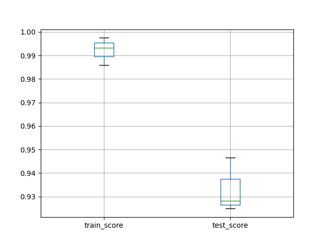
交叉验证调优后管道
前面已经提到,这里的grid是同clf/pipe一样的机器学习模型,自然可以对原数据进行交叉验证
from sklearn.model_selection import cross_validate
import matplotlib.pyplot as plt

scores = cross_validate(grid, X, y, cv=3, n_jobs=1, return_train_score=True)
df_scores = pd.DataFrame(scores)
print(df_scores)
df_scores[['train_score', 'test_score']].boxplot()
plt.show()
2
3
4
5
6
7
8
    fit_time  score_time  test_score  train_score
0  23.017125    0.000651    0.928214     0.985810
1  25.200372    0.000676    0.946578     0.997496
2  23.103306    0.000675    0.924875     0.993322
2
3
4
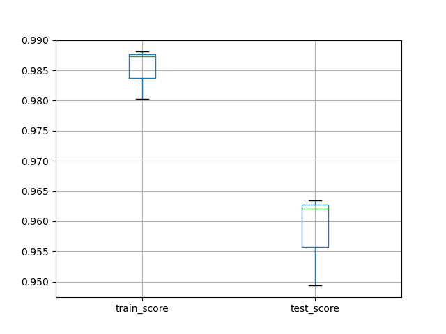
调优训练 breast_cancer
在乳腺癌数据集上对管道进行调优并训练测试
- 导入数据,分割数据
- 构建管道,调优参数
- 训练测试,交叉验证
from sklearn.datasets import load_breast_cancer
from sklearn.metrics import balanced_accuracy_score

X, y = load_breast_cancer(return_X_y=True)

from sklearn.model_selection import train_test_split

X_train, X_test, y_train, y_test = train_test_split(X, y, random_state=12, stratify=y)

from sklearn.pipeline import make_pipeline
from sklearn.linear_model import SGDClassifier
from sklearn.preprocessing import StandardScaler

pipe = make_pipeline(StandardScaler(), SGDClassifier(max_iter=1000))

from sklearn.model_selection import GridSearchCV

param = {'sgdclassifier__loss': ['hinge', 'log'],
         'sgdclassifier__penalty': ['l2','l1']}
grid = GridSearchCV(pipe, cv=3, n_jobs=1, param_grid=param, return_train_score=True)
grid.fit(X_train, y_train)

accuracy = grid.score(X_test, y_test)


from sklearn.model_selection import cross_validate
import pandas as pd
import matplotlib.pyplot as plt

scores = cross_validate(grid, X, y, scoring='balanced_accuracy',
                        cv=3, return_train_score=True)
df_scores = pd.DataFrame(scores)
df_scores[['train_score', 'test_score']].boxplot()
plt.show()

print(grid.best_params_)
print(df_scores)
print("the accuracy is ", accuracy)
2
3
4
5
6
7
8
9
10
11
12
13
14
15
16
17
18
19
20
21
22
23
24
25
26
27
28
29
30
31
32
33
34
35
36
37
38
{'sgdclassifier__loss': 'hinge', 'sgdclassifier__penalty': 'l1'}

   fit_time  score_time  test_score  train_score
0  0.031983    0.000585    0.962067     0.980303
1  0.034171    0.000492    0.949343     0.987261
2  0.032296    0.000593    0.963445     0.988076

the accuracy is 0.9440559440559441
2
3
4
5
6
7
8
管道使用总结
使用scikit-learn十行以内训练并测试一个管道,包括数据预处理、参数调优、交叉验证
import pandas as pd
from sklearn.preprocessing import MinMaxScaler
from sklearn.linear_model import LogisticRegression
from sklearn.pipeline import make_pipeline
from sklearn.model_selection import GridSearchCV
from sklearn.model_selection import cross_validate
from sklearn.datasets import load_digits
import matplotlib.pyplot as plt

X, y = load_digits(return_X_y = True)

pipe = make_pipeline(MinMaxScaler(),
                     LogisticRegression(solver='saga', multi_class='auto', random_state=42, max_iter=5000))
param = {'logisticregression__C': [0.1, 1.0, 10],
        'logisticregression__penalty': ['l2', 'l1']}
grid = GridSearchCV(pipe, param_grid=param, cv=3, n_jobs=-1)
scores = pd.DataFrame(cross_validate(grid, X, y, cv=3, n_jobs=-1, return_train_score=True))
scores[['train_score', 'test_score']].boxplot()

plt.show()
2
3
4
5
6
7
8
9
10
11
12
13
14
15
16
17
18
19
20

Heterogeneous Data
Heterogeneous data
处理除数字以外的数据
导入外部数据集
注意shell的位置,这里找的是当前shell路径的相对路径
- 通过
os.getcwd()获取当前路径(pwd)
import pandas as pd
import os

print(os.getcwd())

data = pd.read_csv(os.path.join('data','titanic_openml.csv'), na_values='?')
print(data.head(7))
print(data.tail(4))
2
3
4
5
6
7
8
先拟合再学习
从原始数据中提取出数据集
- 在该泰坦尼克模型中,自变量为年龄、性别、是否上船、恐惧等因素,因变量为是否存活
分割数据集为训练集和测试集,采用线性回归模型进行学习
y = data['survived']
X = data.drop(columns='survived')

print(y)

from sklearn.model_selection import train_test_split

X_train, X_test, y_train, y_test = train_test_split(X, y, random_state=12)

from sklearn.linear_model import LogisticRegression

clf = LogisticRegression()
clf.fit(X_train, y_train)
2
3
4
5
6
7
8
9
10
11
12
13
- 必然报错,因为
fit方法接收的数据集要求数据为数字型,而这里的很多数据如性别、是否上船并不是数字数据
使用管道处理非数字数据,同时使用管道标准化数字数据,这里实际上都是预处理数据的过程
- 处理非数字数据,即转化为数字数据同时处理缺失数据
SimpleImputer(strategy='constant')OneHotEncoder()
- 标准化数字数据同时处理缺失数据
SimpleImputer(strategy='mean')StandardScaler()
OneHotEncoder示例
from sklearn.impute import SimpleImputer
from sklearn.preprocessing import OneHotEncoder
ohe = make_pipeline(SimpleImputer(strategy='constant'), OneHotEncoder())
X_encoded = ohe.fit_transform(X_train[['sex', 'embarked']])
X_encoded.toarray()
2
3
4
5
[[0. 1. 1. 0. 0. 0.]
 [0. 1. 0. 0. 1. 0.]
 [0. 1. 1. 0. 0. 0.]
 ...
 [0. 1. 0. 0. 1. 0.]
 [1. 0. 0. 0. 1. 0.]
 [0. 1. 1. 0. 0. 0.]]
2
3
4
5
6
7
处理titanic数据
1、提取非数字列和数字列
col_cat = ['sex', 'embarked']
col_num = ['age', 'sibsp', 'parch', 'fare']

X_train_cat = X_train[col_cat]
X_test_cat = X_test[col_cat]
X_train_num = X_train[col_num]
X_test_num = X.test[col_num]
2
3
4
5
6
7
2、构建管道预处理数据
为什么要用管道而不是单独预处理,因为需要同时处理缺失数据
- 数字化非数字数据
- 标准化数字数据
- 处理缺失数据
from sklearn.pipeline import make_pipeline
from sklearn.impute import SimpleImputer
from sklearn.preprocessing import OneHotEncoder
from sklearn.preprocessing import StandardScaler

scaler_cat = make_pipeline(SimpleImputer(strategy='constant'), OneHotEncoder())
scaler_num = make_pipeline(SimpleImputer(strategy='mean'), StandardScaler())

X_train_cat_scaled = scaler_cat.fit_transform(X_train_cat)
X_test_cat_scaled = scaler_cat.transform(X_test_cat)
X_train_num_scaled = scaler_num.fit_transform(X_train_num)
X_tes
2
3
4
5
6
7
8
9
10
11
12
3、合并预处理后的数字数据和非数字数据,采用矩阵横向合并的方法(即合并列为一张大表)
import numpy as np
from scipy import sparse
X_train_scaled = sparse.hstack((X_train_cat_scaled,
                sparse.csr_matrix(X_train_num_scaled)))
X_test_scaled = sparse.hstack((X_test_cat_scaled,
                sparse.csr_matrix(X_test_num_scaled)))
2
3
4
5
6
4、现在已经有完整的数字标准化后的训练、测试数据,直接构建模型开始学习(fit)即可
from sklearn.linear_model import LogisticRegression

clf = LogisticRegression()
clf.fit(X_train_scaled, y_train)
accuracy = clf.score(X_test_scaled, y_test)
print("Accuracy score of the {} is {:.2f}".format(clf.__class__.__name__, accuracy))
2
3
4
5
6
通过管道学习
上述过程可以概括为:
- 预处理数据
- 提取数据的非数字列和数字列
- 通过管道分别数字化、标准化处理非数字、数字数据,同时处理缺失数据
- 合并处理后的数据
- 建立模型学习并测试
和之前的学习一样,上述过程可以揉合到一个管道中进行,即构建一个含有预处理功能和学习功能的管道
这里有一个问题,就是对于数字数据和非数字数据,其预处理的方式并不同,所以管道的预处理功能应该针对特定列有不同的处理方法
这里用到sklearn.compose.make_column_transformer(transformer, col_name)合并多个管道并使之作用于不同列
- 导入数据,独立分割
data = pd.read_csv(os.path.join(), na_values='?')train_test_split
- 构建预处理管道
make_pipeline(空值处理器, 预处理器)
- 合并预处理管道
make_column_transformer((预处理管道, 列名)...)
- 构建总管道
make_pipeline(预处理器, 分类器)
- 学习并测试
fit()/score()
from sklearn import preprocessing
from sklearn.linear_model import LogisticRegression
from sklearn.model_selection import train_test_split
import os
from sklearn.preprocessing import StandardScaler
from sklearn.preprocessing import OneHotEncoder
from sklearn.impute import SimpleImputer
from sklearn.pipeline import make_pipeline
import pandas as pd
import numpy as np

data = pd.read_csv(os.path.join('data','titanic_openml.csv'), na_values='?')
y = data['survived']
X = data.drop(columns='survived')

# print(X)

X_train, X_test, y_train, y_test = train_test_split(X, y, random_state=12)

# print(y_train)

col_cat = ['sex', 'embarked']
col_num = ['age', 'sibsp', 'parch', 'fare']

pre_cat = make_pipeline(SimpleImputer(strategy='constant'), OneHotEncoder(handle_unknown='ignore'))
pre_num = make_pipeline(SimpleImputer(strategy='mean'), StandardScaler())

from sklearn.compose import make_column_transformer

preprocessor = make_column_transformer((pre_cat, col_cat), (pre_num, col_num))
pipe = make_pipeline(preprocessor, LogisticRegression(solver='lbfgs'))
pipe.fit(X_train, y_train)
accuracy = pipe.score(X_test, y_test)
print('Accuracy score of the {} is {:.2f}'.format(pipe.__class__.__name__, accuracy))
2
3
4
5
6
7
8
9
10
11
12
13
14
15
16
17
18
19
20
21
22
23
24
25
26
27
28
29
30
31
32
33
34
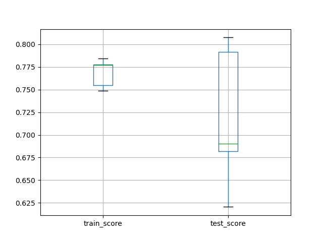
优化管道参数
在上述包含预处理功能和学习功能的管道的基础上,在正式测试之前使用网格搜索GridSearchCV对其参数进行调优
from sklearn.model_selection import GridSearchCV
from sklearn.model_selection import cross_validate
import pandas as pd
import matplotlib.pyplot as plt

# 调优参数
param = {'columntransformer__pipeline-2__simpleimputer__strategy': ['mean', 'median'],
        'logisticregression__C': [0.1, 1.0, 10]}
grid = GridSearchCV(pipe, param_grid=param, cv=5, n_jobs=1)

grid.fit(X_train, y_train)
print(grid.score(X_test, y_test))
# 交叉验证得分
scores = cross_validate(grid, X, y, scoring='balanced_accuracy', cv=5, n_jobs=-1, return_train_score=True)
# 绘制箱型图
df_scores = pd.DataFrame(scores)
df_scores[['train_score', 'test_score']].boxplot()
plt.show()
2
3
4
5
6
7
8
9
10
11
12
13
14
15
16
17
18
adult_openml.csv
使用同样的方法处理adult_openml数据集
预处理再拟合
import os
import pandas as pd


data = pd.read_csv(os.path.join('data', 'adult_openml.csv'), na_values='?')
# print(data.head(7))

y = data['class']
X = data.drop(columns=['class', 'fnlwgt', 'capitalgain', 'capitalloss'])

from sklearn.model_selection import train_test_split

X_train, X_test, y_train, y_test = train_test_split(X, y, random_state=12)
# print(y_train)

col_cat = ['workclass', 'education', 'marital-status', 'relationship', 'race', 'sex', 'native-country']
col_num = ['age', 'education-num', 'hoursperweek']

X_train_cat = X_train[col_cat]
X_test_cat = X_test[col_cat]
X_train_num = X_train[col_num]
X_test_num = X_test[col_num]

from sklearn.preprocessing import KBinsDiscretizer
from sklearn.preprocessing import StandardScaler
from sklearn.preprocessing import OneHotEncoder
from sklearn.impute import SimpleImputer
from sklearn.pipeline import make_pipeline


cat_pipe = make_pipeline(SimpleImputer(strategy='constant'), OneHotEncoder())
num_pipe = make_pipeline(SimpleImputer(strategy='mean'), StandardScaler())

X_train_cat_scaled = cat_pipe.fit_transform(X_train_cat)
X_test_cat_scaled = cat_pipe.transform(X_test_cat)
X_train_num_scaled = num_pipe.fit_transform(X_train_num)
X_test_num_scaled = num_pipe.transform(X_test_num)

import numpy as np
from scipy import sparse

X_train_scaled = sparse.hstack((X_train_cat_scaled,
                sparse.csr_matrix(X_train_num_scaled)))
X_test_scaled = sparse.hstack((X_test_cat_scaled,
                sparse.csr_matrix(X_test_num_scaled)))

from sklearn.linear_model import LogisticRegression

clf = LogisticRegression(max_iter=1000)
clf.fit(X_train_scaled, y_train)
accuracy = clf.score(X_test_scaled, y_test)
print('accuracy of the {} is {:.2f}'.format(clf.__class__.__name__, accuracy))
2
3
4
5
6
7
8
9
10
11
12
13
14
15
16
17
18
19
20
21
22
23
24
25
26
27
28
29
30
31
32
33
34
35
36
37
38
39
40
41
42
43
44
45
46
47
48
49
50
51
52
accuracy of the LogisticRegression is 0.83
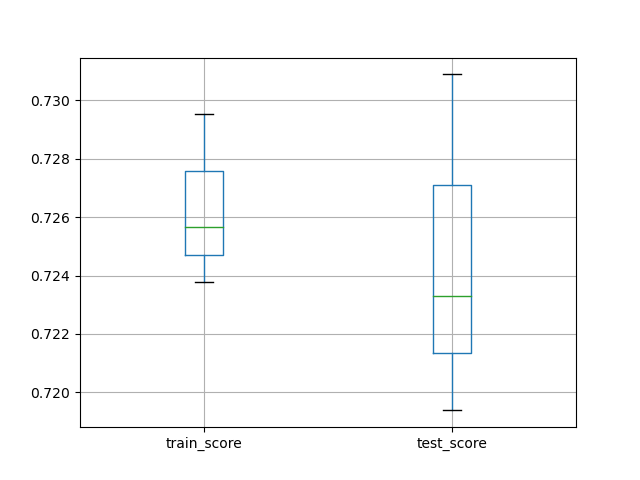
优化管道处理
import os
import pandas as pd

data = pd.read_csv(os.path.join('data', 'adult_openml.csv'), na_values='?')
# print(data.head(3))
y = data['class']
X = data.drop(columns=['class', 'fnlwgt', 'capitalgain', 'capitalloss'])
# print(X)

from sklearn.preprocessing import LabelEncoder
from sklearn.model_selection import train_test_split

X_train, X_test, y_train, y_test = train_test_split(X, y, random_state=12)
# print(y_train)
encoder = LabelEncoder()
y_train = encoder.fit_transform(y_train)
y_test = encoder.transform(y_test)

from sklearn.pipeline import make_pipeline
from sklearn.impute import SimpleImputer
from sklearn.preprocessing import StandardScaler
from sklearn.preprocessing import OneHotEncoder
from sklearn.compose import make_column_transformer
from sklearn.linear_model import LogisticRegression
from sklearn.model_selection import GridSearchCV

pre_cat = make_pipeline(SimpleImputer(strategy='constant'), OneHotEncoder(handle_unknown='ignore'))
pre_num = make_pipeline(SimpleImputer(strategy='mean'), StandardScaler())

col_cat = ['workclass', 'education', 'marital-status', 'relationship', 'race', 'sex', 'native-country']
col_num = ['age', 'education-num', 'hoursperweek']

preprocessor = make_column_transformer((pre_cat, col_cat), (pre_num, col_num))
# preprocessor.fit(X_train, y_train)

pipe = make_pipeline(preprocessor, LogisticRegression(solver='lbfgs', max_iter=5000))
# pipe.fit(X_train, y_train)

param = {'logisticregression__C': [0.1, 1.0, 10]}
grid = GridSearchCV(pipe, param_grid=param, cv=5, n_jobs=1)
grid.fit(X_train, y_train)
accuracy = grid.score(X_test, y_test)
print('accuracy of the {} is {:.2f}'.format(grid.__class__.__name__, accuracy))

from sklearn.model_selection import cross_validate
import matplotlib.pyplot as plt
scores = pd.DataFrame(cross_validate(grid, X, y, scoring='balanced_accuracy', cv=3, n_jobs=-1, return_train_score=True))
print(scores)
scores[['train_score', 'test_score']].boxplot(whis=10)
plt.show()
2
3
4
5
6
7
8
9
10
11
12
13
14
15
16
17
18
19
20
21
22
23
24
25
26
27
28
29
30
31
32
33
34
35
36
37
38
39
40
41
42
43
44
45
46
47
48
49
50
accuracy of the GridSearchCV is 0.83

    fit_time  score_time  test_score  train_score
0  11.303147    0.064652    0.719383     0.729532
1  12.427096    0.067366    0.730889     0.723769
2  12.042301    0.078128    0.723290     0.725647
2
3
4
5
6